Robotic Arm Simulation
CMPUT 340: Numerical Methods & Optimization • University of Alberta
View Source on GitHubInteractive 2D robotic arm simulation implementing inverse kinematics, analytical and finite-difference Jacobians, Newton's method, and Broyden's quasi-Newton numerical optimization.
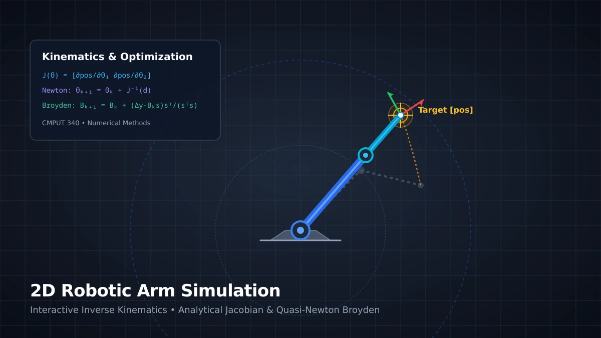
In robotics and computer graphics, controlling multi-link mechanisms requires solving the Inverse Kinematics (IK) problem: given a target Cartesian coordinate (x*, y*) in workspace coordinates, determine the exact joint angles (θ1, θ2) required for the arm's end-effector to reach that point.
Because forward kinematics maps angles through transcendental trigonometric equations, inverse kinematics yields a system of non-linear equations. In this project, I developed an interactive 2D simulation in MATLAB and ported the core algorithms to interactive TypeScript and HTML5 Canvas. We explore both an exact gradient-based solver (Newton's Method) and a memory-efficient secant update (Broyden's Quasi-Newton Method), analyzing convergence speed, Jacobian evaluation costs, and numerical stability near kinematic singularities.
Project Summary
Core Competencies
- Non-Linear Root Finding & Numerical Optimization
- Analytical Jacobian Derivation & Sensitivity Analysis
- Finite-Difference Approximations & Round-Off Error
- Newton-Raphson vs. Broyden's Quasi-Newton Method
- Damped Least Squares & Kinematic Singularity Handling
Quick Facts
- Course: CMPUT 340 (Numerical Methods)
- Degrees of Freedom: 2-DOF Planar Arm
- Languages: MATLAB, TypeScript, HTML5 Canvas
- Convergence Rate: Quadratic (Newton) vs. Superlinear (Broyden)
Interactive Simulation
Click or drag anywhere in the workspace below to position the target point. Toggle between Newton's method (exact or finite-difference) and Broyden's quasi-Newton solver, or compare both solvers side-by-side to observe convergence paths in real time.
Tolerance threshold: ε = 0.001
End-Effector: (0.380, 0.520)
det(J) = 0.2463
Newton: exact analytical derivatives
Kinematic & Numerical Tuning
1. Kinematic Modeling
Consider a planar two-link manipulator rooted at the Cartesian origin (0, 0) with link lengths l1, l2 and joint rotation angles θ1, θ2. The angle θ1 is measured relative to the global horizontal x-axis, while θ2 represents the relative angle of the second link with respect to the first link.
The forward kinematics map F: ℝ² → ℝ² computes the Cartesian position (x, y)ᵖ of the end-effector from joint space coordinates:
y(θ) = l₁ · sin(θ₁) + l₂ · sin(θ₁ + θ₂)
Given a desired end-effector target position pos* = (x*, y*)ᵖ, inverse kinematics seeks joint angles θ = (θ1, θ2)ᵖ that satisfy the non-linear vector equation:
2. The Jacobian Matrix: Analytical vs. Finite-Difference
The Jacobian matrix J(θ) ∈ ℝ²×² is the matrix of all first-order partial derivatives of the forward kinematics function. It describes how infinitesimal variations in joint angles produce linear displacements in Cartesian space:
[ ∂y/∂θ₁ ∂y/∂θ₂ ]
Differentiating the forward kinematics equations with respect to each joint angle yields the exact analytical Jacobian:
∂x/∂θ₂ = -l₂·sin(θ₁ + θ₂)
∂y/∂θ₁ = l₁·cos(θ₁) + l₂·cos(θ₁ + θ₂)
∂y/∂θ₂ = l₂·cos(θ₁ + θ₂)
Central Finite-Difference Approximation
In more complex multi-body robotic systems (such as 6-DOF industrial manipulators or tendon-driven continuum arms), deriving and computing symbolic analytical derivatives can be cumbersome or computationally expensive. We implemented a central finite-difference approximation with perturbation step h:
∂F/∂θ₂ ≈ ( F(θ + [0; h]) - F(θ - [0; h]) ) / (2h)
Perturbation Trade-Off: Truncation vs. Round-Off Error
The truncation error of central differences scales as O(h²), meaning smaller h yields higher mathematical fidelity. However, as h → 0, floating-point cancellation errors scale as O(εmach / h). In MATLAB (IEEE 754 double precision), values such as h = 0.01 or h = 10-4 yield accurate gradients without catastrophic cancellation, whereas large values (e.g., h = 0.5) introduce noticeable directional drift into the solver iterations.
3. Inverse Kinematics Solvers: Newton vs. Broyden
To iteratively find joint angles θ that drive the end-effector error d = pos* - F(θ) below a specified tolerance threshold (ε = 0.001), two primary numerical optimization strategies were implemented and evaluated:
Method 1: Newton-Raphson Method
At each iteration step k, Newton's method forms a local linear Taylor approximation of the kinematic mapping and solves the linear system for the angular correction step sk:
θᵢ₊₁ = θᵢ + sᵢ
Newton's method demonstrates quadratic local convergence when the initial guess is sufficiently close to the solution. However, it requires recalculating the entire Jacobian matrix at every iteration, which for high-DOF arms or complex forward kinematic models can become the dominant computational bottleneck.
Method 2: Broyden's Quasi-Newton Method
Broyden's method generalizes the 1D secant method to multiple dimensions. Rather than evaluating fresh derivatives at every iteration, Broyden begins with an initial Jacobian estimate B0 (evaluated once at θ0) and updates the matrix iteratively using the minimum Frobenius-norm rank-1 correction that satisfies the secant condition:
where sk = θk+1 - θk is the joint step and yk = f(θk+1) - f(θk) is the change in residual error.
Newton's Method
- Convergence: Quadratic (||ek+1|| ≤ C ||ek||²)
- Iterations: Typically 3–5 iterations
- Cost per step: High (recomputes full Jacobian J)
- Sensitivity: Sensitive to initial guess and singularities
Broyden's Method
- Convergence: Superlinear
- Iterations: Typically 6–10 iterations
- Cost per step: Low (simple vector outer product update)
- Sensitivity: Slower to track rapid curvature changes
4. Kinematic Singularities & Damped Least Squares
A kinematic singularity occurs when the manipulator loses one or more degrees of freedom, causing the Jacobian matrix to lose rank. For our 2D planar arm, the determinant of the Jacobian is:
Singularities occur when θ2 = 0 (arm completely outstretched at the workspace boundary R = l1 + l2) or θ2 = π (arm completely folded in on itself). When det(J) → 0, naive matrix inversion produces unbounded angular velocities (sk → ∞).
To prevent numerical blow-ups when users test near-singular postures, we introduced a Damped Least Squares (Levenberg-Marquardt) regularization:
The damping parameter λ ≈ 0.05 smoothly limits step magnitudes near singular configurations, ensuring graceful degradation rather than erratic numerical oscillations.
5. Original MATLAB Implementation
Below are excerpts from the original MATLAB script developed for CMPUT 340, highlighting the forward kinematics, finite-difference approximation, and iterative inverse kinematics routine:
function [pos, J] = evalRobot2D(l, theta)
    l1 = l(1);
    l2 = l(2);
    th1 = theta(1);
    th2 = theta(2);

    x = l1*cos(th1) + l2*cos(th1 + th2);
    y = l1*sin(th1) + l2*sin(th1 + th2);
    pos = [x; y];

    dx_dth1 = -l1*sin(th1) - l2*sin(th1 + th2);
    dx_dth2 = -l2*sin(th1 + th2);
    dy_dth1 =  l1*cos(th1) + l2*cos(th1 + th2);
    dy_dth2 =  l2*cos(th1 + th2);

    J = [dx_dth1, dx_dth2; dy_dth1, dy_dth2];
endfunction J = fdJacob2D(l, theta, h)
dpos_dtheta1 = ( evalRobot2D(l, theta+[h;0]) - evalRobot2D(l, theta-[h;0]) ) / (2*h);
dpos_dtheta2 = ( evalRobot2D(l, theta+[0;h]) - evalRobot2D(l, theta-[0;h]) ) / (2*h);
J = [dpos_dtheta1, dpos_dtheta2];
endfunction theta = invKin2D(l, theta0, pos, n, mode)
tol = 0.001; % Tolerance threshold
if mode == 0
% Broyden's Quasi-Newton Method
theta = theta0;
[current_pos, J] = evalRobot2D(l, theta); % Initial Jacobian
d = current_pos - pos;
for k = 1:n
if norm(d) < tol
break;
end
s_k = -J \ d;
theta = theta + s_k;
[new_pos, ~] = evalRobot2D(l, theta);
d_new = new_pos - pos;
y_k = d_new - d;
% Rank-1 Broyden update
J = J + ((y_k - J * s_k) * s_k') / (s_k' * s_k);
d = d_new;
end
elseif mode == 1
% Newton's Method
theta = theta0;
for k = 1:n
[current_pos, J] = evalRobot2D(l, theta);
d = pos - current_pos;
if norm(d) < tol
break;
end
s_k = J \ d;
theta = theta + s_k;
end
end
end6. Key Conclusions & Insights
Through experimental testing of both solvers across various workspace configurations, several core insights emerged:
- Initial Guess Matters: Because the inverse kinematics mapping has multiple solutions (elbow-up vs. elbow-down configurations) and local minima outside the reachable workspace, both Newton and Broyden depend on a reasonable initial posture θ0.
- Broyden Minimizes Function Calls: When the forward kinematics evaluation is computationally expensive, Broyden's method is vastly superior per second of CPU time, even though it requires roughly 1.5x to 2x more iteration steps than Newton's method.
- Exact Jacobians Accelerate Terminal Convergence: Once within the basin of attraction, Newton's method achieves machine precision in just a few steps, doubling the number of correct significant digits with each step due to quadratic convergence.